What Is Phase Coherence Imaging (PCI)?
Phase Coherence Imaging (PCI) is a phased array ultrasonic imaging method that forms an image by evaluating how consistent the signal phase is across multiple emitter-receiver pairs in an FMC dataset. Unlike amplitude-focused imaging (such as TFM), PCI emphasizes indications that remain phase-consistent across many paths, which often corresponds to omnidirectional scattering sources. In practice, this can enhance porosity/slag and crack tip diffraction responses while reducing strong geometry echoes from the front surface and backwall. PCI values depend strongly on reflector type and orientation, so method selection should be application-driven.
How to Calculate a PCI Image
What you will learn in this section:
You will learn what data PCI needs (FMC), how PCI differs from TFM in terms of what it sums (phase vs amplitude), and what the PCI value represents at a pixel.
Key idea:
TFM sums amplitudes at each pixel after applying time-of-flight delays; PCI follows the same time-of-flight logic but sums phase-consistent contributions instead of amplitude.
Here we’ll explain how to calculate a Total Focusing Method (TFM) image first. The FMC/TFM is an inspection technique that involves two steps. The first is the data acquisition process called FMC, and the second is data reconstruction: TFM. The whole process is typically done in real time on most hardware, so the two steps are transparent to users.
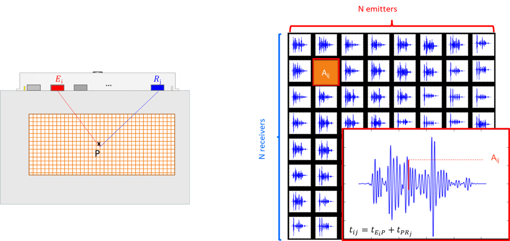
The FMC is a matrix consisting of the combination of N transmitted signals and N received signals with each matrix cell containing an A-scan time domain signal. It is obtained by firing the N elements of the Phased Array Ultrasonic Testing (PAUT) probe one by one and recording on all receivers each time.
The TFM algorithm consists of coherently summing amplitudes from the signals of the FMC dataset to focus at every pixel of a Region of Interest (ROI). Mathematically, this can be expressed as:
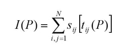
Where tij(P) denotes the theoretical time-of-flight corresponding to the propagation time between the emitter Ei and receiver Rj, through one of the pixels P.
The following figure explains the process for one pixel and one signal of the FMC.
-
The TFM process calculates the time-of-flight tij to go from emitter Ei to pixel P and back to receive Rj. The amplitude Aij corresponding to that time-of-flight is then extracted for that particular signal.
-
The process is then repeated for all the signals of the FMC matrix.
-
All these amplitudes are summed, and the result is the amplitude for that pixel in the TFM image.
-
The entire process is then repeated for all the pixels to obtain the TFM image.
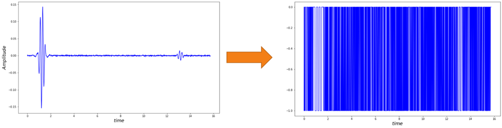
To calculate the PCI image, we need to transform the A-scan signals of the FMC into phase versus time. The phase can be obtained by dividing the signals by the modulus of their Hilbert transform (analytical signal). An alternative is to extract the sign of the FMC signals. It provides similar results as calculating the true phase and has a simpler implementation on the hardware. Each signal of the FMC matrix is replaced by its sign function so each data point is either a 1 or -1.
The process for calculating the PCI image is then similar to the TFM one. We calculate the time-of-flight tij to go from emitter Ei to pixel P and back to receive Rj. The phase Øij corresponding to that time-of-flight is then extracted for that particular signal. The process is then repeated for all the signals (transformed into their sign version) of the FMC matrix. All these phases are summed and the result is the phase for that pixel in the PCI image. The entire process is then repeated for all the pixels to obtain the PCI image.
PCI Intensity Explanation
Direct Interpretation (what a high or low PCI value means)
A high PCI value indicates that many emitter-receiver pairs contribute with a similar phase at that pixel, which is typical of omnidirectional scatterers and crack tip diffractions. A low PCI value often indicates phase that varies strongly with direction, which is common for geometry echoes (front surface, backwall) and some specular planar reflectors depending on their orientation and position.
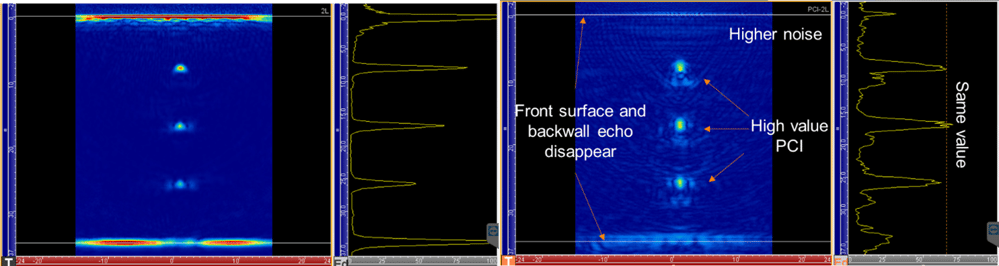
If we compare the PCI image obtained on a mockup containing three side-drilled holes (SDH) to the TFM one, we can observe that:
-
PCI pretty much removes the front surface and backwall echoes,
-
The PCI value for the three SDH is identical,
-
The noise level in the PCI image is higher.
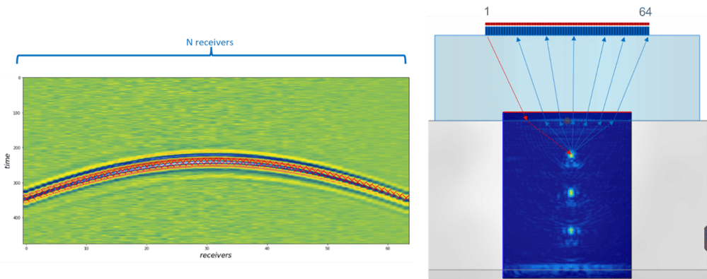
Why do we obtain high values for the SDH and low values for the geometry echoes? First let’s look at the pixel located at the maximum of the first SDH. In the image on the left, we display the first column of the FMC matrix, i.e., the 64 received signals after firing the first element. On top of that we superimpose the times-of-flight (red crosses) to go from emitter one to the SDH back to all the receivers. We can see that the red crosses superimpose perfectly for the same phase on all receivers, meaning that all the signals are in phase. By summing all these contributions, we obtain a high PCI value.
With the same reasoning for the pixel located in the middle of the backwall, we display the B-scan obtained after firing the first element and the times-of-flight to go from emitter one to the middle of the backwall back to all receivers (red crosses). Looking at the red crosses, we can see that they are superimposed with the same phase only for the last receivers (indicated by the red rectangle).
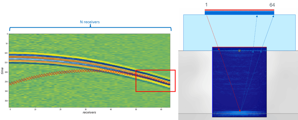
When dealing with geometry echoes such as front surface and backwall, mostly the symmetric paths contribute to the PCI image. All the other paths lead to an incoherent sum, which explain the low values of the PCI image along the backwall and front surface echo. This can be the same for other specular reflectors like delamination or lack of fusion depending on their position with respect to the probe.
When dealing with amplitude signals, the Signal-to-Noise Ratio (SNR) can be relatively high depending on the nature of the indications (backwall, LOF, etc.). The more energy we send into the part, by increasing the voltage of the analog gain for example, the better the SNR is for a TFM image. For phase signals, the noise varies between -1 and 1 like the phase of indications even if more energy is sent into the part.
Practical Rule: SNR Improves with the Number of Sources
In PCI, noise and indications both map to phase-like values, so increasing energy (gain/voltage) does not improve SNR the same way it does in amplitude imaging. A practical way to improve PCI stability is to increase the number of emitter-receiver pairs used in the sum. This is why full FMC often provides more stable PCI images than sparse FMC.
If you want a conservative lower threshold for display dynamic range, you can estimate the probability of noise excursions because the summed values behave like a distribution of +1 and -1 contributions.
Example thresholding insight (from this dataset):
- With full FMC (4096 signals), noise levels above roughly 6% are very unlikely across a 500k-pixel PCI image.
- With sparse FMC (1024 signals, 16 emissions), noise levels above roughly 11% are very unlikely.
These values can help operators set a conservative lower threshold for the display dynamic range, while recognizing that rare higher excursions can still occur.
![]()
Results Obtained for Normal Incidence Inspections
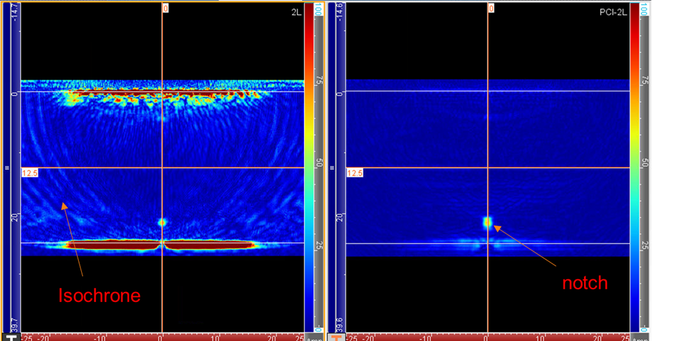
In our first example, we look at a 25-millimeter-thick mockup with a notch along the backwall. We are using a 64L5-G3 probe with a 20-millimeter (0.787-inch) L0 wedge. We calculate at the same time the TFM and PCI images displayed below. We can see some artifacts in the TFM image called isochrones. When we calculate the times-of-flight to go to pixels covered by those artifacts, some of the TOF in the FMC matrix corresponds to contributions from the backwall; so, when we sum those contributions, we obtain some signal. The presence of those artifacts depends on the thickness of the part and the pitch. Looking at the PCI image, we see that those artifacts are gone as they are contributions from the backwall, and PCI tends to remove geometry echoes. We can see the tip of the notch very clearly, allowing perfect detection and sizing.
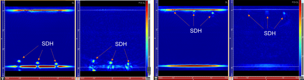
PCI is very efficient at seeing defects close to the backwall. We can see in the following figure on the left three SDH close to the backwall for TFM and PCI. PCI detects them while removing the backwall, which would allow detection much closer to it. It is not necessarily better than TFM when it comes to defects close to the front surface despite removing the front surface echo. If we look at the image on the right, we can distinguish two of the SDH in the TFM image, the other one being in the dead zone. For PCI, we see the deepest SDH and distinguish the middle one. This is due to the fact that a lot of the emitter-receiver pairs far from the defect don’t contribute in phase.
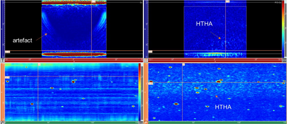
A perfect application for PCI is the inspection of High Temperature Hydrogen Attack (HTHA). HTHA damage usually displays small cracks that send energy in all directions. Eddyfi Technologies developed a 64-element, 10-MHz probe that focuses along the passive plane to improve sensitivity as cracks are small in both directions. The sample that we looked at has micro-cracks ranging from a few microns to less than 100 microns. The following image shows the TFM with its C-scan on the left and the PCI on the right. The TFM image shows the same artifacts as we have seen before preventing the detection of the very tiny microcracks. The PCI image removes the artifacts and shows tiny responses along the backwall corresponding to the HTHA damage. Looking at the C-scan, we can clearly see the cloud of HTHA, which is not visible on the TFM image.
FMC
PWI
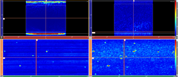
One drawback of PCI is the need to use a full FMC to obtain a good SNR. This usually has an impact on productivity. We have implemented Plane Wave Imaging (PWI) in the past to improve scanning speed for TFM inspections. We have applied PWI combined with PCI using 16 angles ranging from -20 to 20° to the same HTHA mockup, and we obtained the same results despite the fact that we used four times less sources. In theory, our noise level should have pretty much doubled. What’s happening here is that some of the FMC A-scans didn’t have enough energy as the defects are really tiny, and their SNR was zero. It is not possible to extract a phase when there is no signal. PWI allowed for sending more energy into the part and obtaining sufficient energy to extract a phase compensating for the increased noise due to the fact that we only used 16 sources. This allows increasing the scanning speed by a factor close to four.
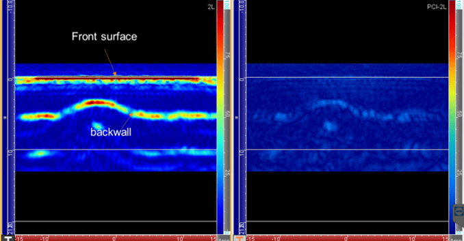
We also looked at corrosion mapping and composite inspection, both of which are usually performed with a normal incidence inspection. We compare it to TFM using the same probe described before. For corrosion, TFM shows the front surface echo and the backwall allowing measurement of the remaining wall thickness. As PCI removes the front surface and backwall echoes and doesn’t have good detectability close to the front surface, it is not the best technique for corrosion mapping. We can distinguish a little bit the backwall with PCI, but it mostly shows areas where there is changes of slope as diffraction echoes. The front surface is completely gone.
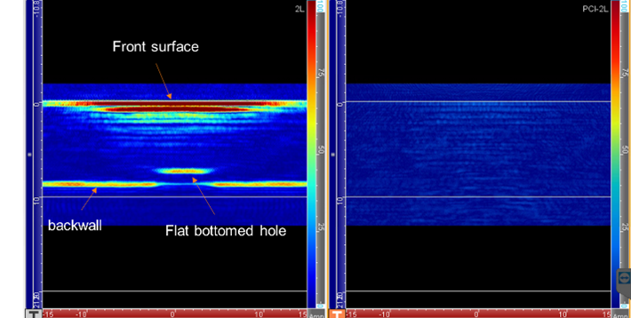
It is similar for composite inspection for which the front surface and backwall echoes disappear entirely as well as the Flat-Bottomed Hole (FBH). In composite material inspection, it is difficult for the ultrasound to propagate at an angle as the plies steer the energy either perpendicularly or along the plies. For PCI, mostly the symmetric paths contribute, i.e., the ones with the most angle. This explains why the backwall and FBH are completely gone.
Results Obtained for Angled Beam Inspections
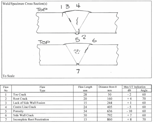
We looked at applying PCI to weld inspection. We inspected a carbon steel pipe containing seven defects. The solution-based manual UT scanner is in its weld inspection configuration. We used two 64L5-G3 probes with SW55 wedge.
We performed multiple inspections in a multigroup configuration comparing TFM to PCI using a full FMC, sparse FMC and PWI.
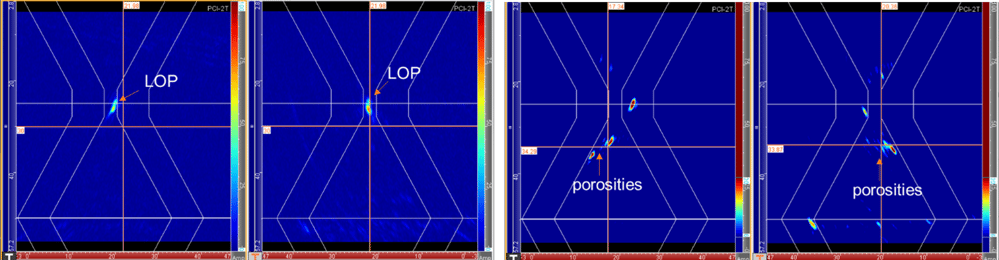
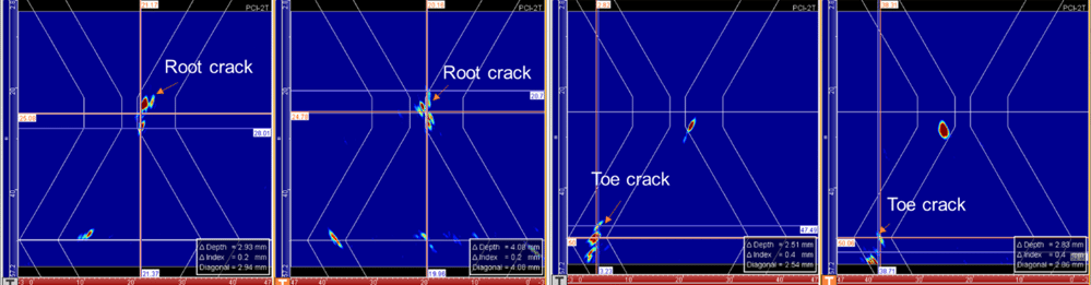
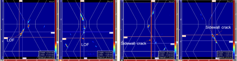
In the following figures, we display the various defects obtained with PCI on each side of the probe, no TFM here, for all the defects. The dynamic range is adjusted between 6%, which is the theoretical value for the noise when using a full FMC, and 30% to increase the visualization of the weaker PCI values.
Volumetric defects like porosities are easily detected with an SNR of 19 dB. The root and toe crack are detected from both sides and lead to tip diffraction for characterization. Some discrepancies appear in terms of sizing when comparing from both sides. This could be caused by rebound off the root of the weld. In the same way, we can see that the lack of fusion and the sidewall crack leads to tip diffraction echoes from both sides. Sizing again shows some discrepancies when looking from both sides. This suggests that inspection from both sides is mandatory to perform accurate sizing.
When performing PCI inspection with multiple groups and a full FMC, the major difficulty is the scanning speed. We evaluated the possibility of using PWI with PCI for the inspection of this weld using only eight angles, which provides an improvement in scanning speed by a factor of eight.
The following shows the LOF obtained with a full FMC (left) and PWI (right). The SNR drops from 22 dB for FMC to 12 dB with PWI. While this is still sufficient to detect tip diffraction echoes and perform sizing in this case, that might not always be the case. It is up to operators to evaluate the necessary number of angles to obtain sufficient SNR on a calibration block containing artificial defects.
%20and%20PWI%20(right).png?width=999&height=259&name=LOF%20obtained%20with%20a%20full%20FMC%20(left)%20and%20PWI%20(right).png)
Warning
We looked at another sample containing a LOF and performed an inspection using TFM and PCI. The TFM image shows a specular reflection, and sizing is possible with a decibel drop. We would expect PCI to show two tip diffractions but it shows only one echo. As it is a non-amplitude-based imaging technique, a decibel drop cannot be used, and the defect cannot be sized. This effect can happen if the LOF is relatively smooth and the probe is positioned in such a way that the angle hitting the bevel perpendicularly (for example, 60° here) hits the defect in the middle. For this position, the LOF acts like geometry echoes with symmetric paths contributing in the middle of the defect.
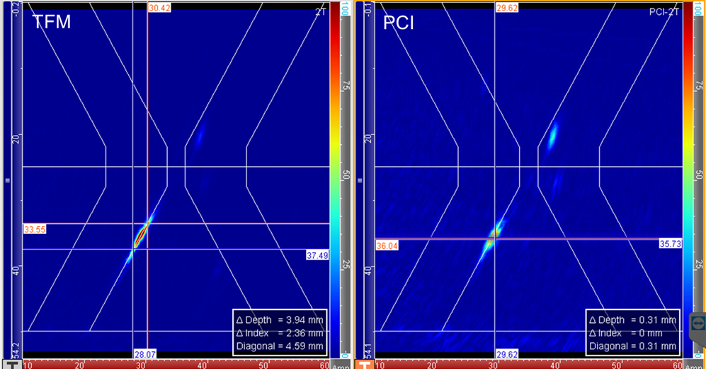
The other discrepancy observed is the difference in sizing when performed on the first and second legs. For example, in the following image we size a LOF using tip diffraction echoes on the first (right) and second (left) legs by positioning cursors along the tip diffraction. We measure a defect height of 5 and 3.9 millimeters (0.197 and 0.154 inches), respectively. The difference could be due to a backwall that is not perfectly parallel to the front surface, UT beam effects, etc. More investigation is required to determine the origin of this discrepancy.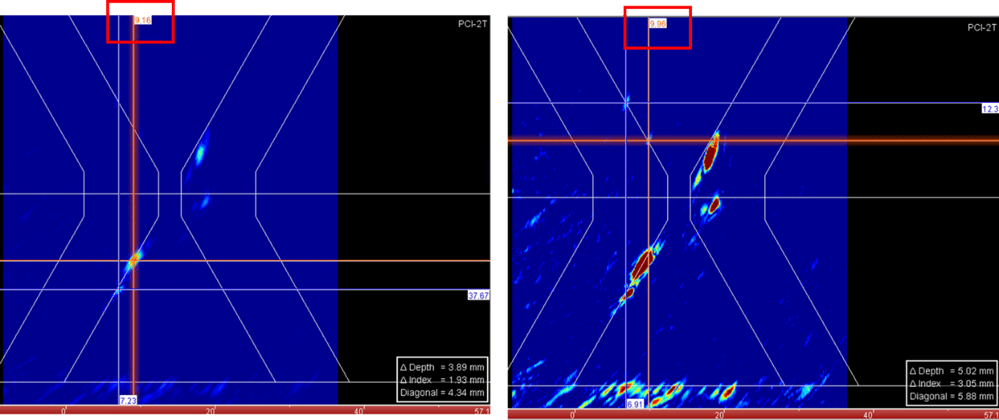
When to Use PCI vs Alternatives (TFM, PWI, Conventional PAUT)
Choose PCI when your primary goal is to enhance phase-consistent indications such as porosity/slag or to make crack tip diffraction easier to interpret for sizing. PCI is often strongest for small indications close to the backwall because it can suppress backwall echoes that mask weak responses in amplitude-based images.
Do not choose PCI when your decision depends on front surface and backwall/interface echoes (for example corrosion mapping or many composite inspections), because PCI can reduce those echoes and degrade thickness or interface interpretation.
| Goal | Best first choice | Why | Key caveat |
|---|---|---|---|
| Detect small volumetric defects (porosity/slag) | PCI + TFM side-by-side | PCI enhances omnidirectional scatterers | Needs enough sources for SNR |
| Size cracks using tip diffraction | PCI (with TFM context) | Tip diffraction can be clearer in PCI | Smooth reflectors may not diffract reliably |
| Detect small indications close to the backwall | PCI + TFM | PCI can suppress backwall masking | Validate on representative calibration |
| Maximize scan speed | PWI-assisted PCI/TFM | Faster acquisition than full FMC | Angle set can reduce SNR |
| Corrosion mapping / wall loss | Conventional UT/PAUT or thickness-oriented TFM | Requires front/backwall echoes | PCI is not recommended |
| Composite inspection | Application-specific UT methods | Interfaces and ply behavior matter | PCI often removes key echoes |
PCI + PWI: how to validate the angle set
If you use PWI to accelerate PCI, validate the minimum angle range and count on a representative mockup: confirm detectability of your smallest target defects and confirm that image noise remains below your chosen display threshold. If SNR is not adequate, increase the number of angles or revert to full FMC for the critical zones.
Pros and Cons of Phase Coherence Imaging
Pros
- Better sizing when tip diffraction is present: PCI can improve sizing for some lack of fusion and fusion-face cracks because crack tip diffraction echoes can be easier to resolve.
- Improved visualization of volumetric defects without gain increases: Porosity and slag can appear with higher relative visibility in PCI compared with amplitude-only imaging.
- Less sensitivity to orientation along the passive plane: PCI can remain effective when reflector responses vary with passive-plane orientation.
- Backwall-adjacent detection advantage: By reducing geometry artifacts, PCI can improve detection of small indications close to the backwall in low-angle or near-normal incidence inspections (for example early-stage HTHA).
- No amplitude calibration for sizing by diffraction: When sizing is based on measuring tip diffraction location, PCI does not rely on amplitude-based calibration curves.
Cons and limitations
- SNR depends on the number of sources: Full FMC is often recommended for stable PCI, which can reduce scanning speed, especially if you must inspect from both sides. PWI can help, but you must tune the number of angles to maintain acceptable SNR.
- Tip diffraction is not guaranteed: Some smooth reflectors (including some LOF conditions) may not produce reliable tip diffraction, making PCI sizing unreliable. In such cases, probe positioning and index offset adjustments may be required, or an alternative sizing approach may be needed.
- Not suited for corrosion mapping and most composite inspections: PCI can suppress front surface and backwall/interface echoes that are essential for thickness or interface interpretation.
- Near-front-surface performance can be weak: Defects close to the front surface may not be detected as reliably as in amplitude-focused methods.
Practical Implementation Checklist (PCI in the field)
Use this checklist to reduce false calls and avoid misapplying PCI:
Setup
- Define the target defect types (volumetric vs planar, expected tip diffraction or not).
- Confirm that the inspection objective does not require front/backwall echoes (avoid PCI for corrosion mapping).
- Choose probe and frequency for your smallest target (higher frequency for micro-cracking when attenuation allows).
Acquisition
- Prefer full FMC for critical zones when SNR is a concern.
- If using PWI, validate the angle range and count on a representative mockup before production scanning.
- Keep acquisition consistent (couplant, wedge, lift-off, scanning speed) to stabilize phase behavior.
Interpretation
- Interpret high PCI values as phase-consistent contributions, not as amplitude.
- Use PCI and TFM side-by-side: PCI for visibility and diffraction cues, TFM for amplitude context and geometry awareness.
- Set display thresholds based on expected noise behavior and confirm on defect-free zones.
Validation and reporting
- Validate detectability and sizing against representative calibration or mockups.
- For weld sizing, consider inspection from both sides when required for reliable tip diffraction visibility.
- Document acquisition mode (FMC vs PWI), angle set, and thresholding approach in the report.
Eddyfi Technologies will propose the PCI technique for the Cypher® portable phased array instruments. It will be possible to use multigroup configurations to simultaneously perform TFM and PCI and combine it with PWI for faster acquisitions. This will allow users to tackle all kinds of applications and evaluate the technology for their own applications.
Take a closer look at easily the most advanced portable PAUT instrument here.
Did you know we offer courses on our advanced PAUT and TFM inspection solutions? Check out the Eddyfi Academy to stay Beyond Current! And for access to instant pricing, contact our experts today.

References:
-
Camacho, M. Parrilla, C. Fritsch, “Phase Coherence Imaging”, IEEE Trans. Ultrason. Ferroelectr. Freq. Control, 56, 5, pp. 958-974, 2009
-
Camacho, D. Atehortua, JF Cruza, J. Brizuela, K. Ealo, “Ultrasonic crack evaluation by phase coherence processing and TFM and its application to online monitoring in fatigue tests”, NDT & E International, Volume 93, Pages 164-174, 2018
-
Lesage, M. Marvasti and O. Farla, “Phase coherence total focusing method for enhancement of small omni-directional scatterers and suppression of geometric reflectors: Application to near-surface crack sizing and detection of high temperature hydrogen attack”, NDT & E International, Volume 123, 2021
-
Dupont-Marillia, J; W. Krynicki, P. Belanger, “Early detection of high temperature hydrogen attack using the ultrasonic full matrix capture and advanced post-processing methods”, NDT&E International 130 (2022)